Size Distributions

DGFit has different functional forms for size distributions that can be used when fitting observed data.

Arbitrary

This is the most flexible size distribution where each size bin is a separate parameter. The total number of parameters is equal to the sum of the number of size distributions for all the different grain compositions.

MRN

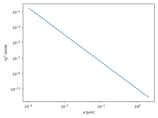
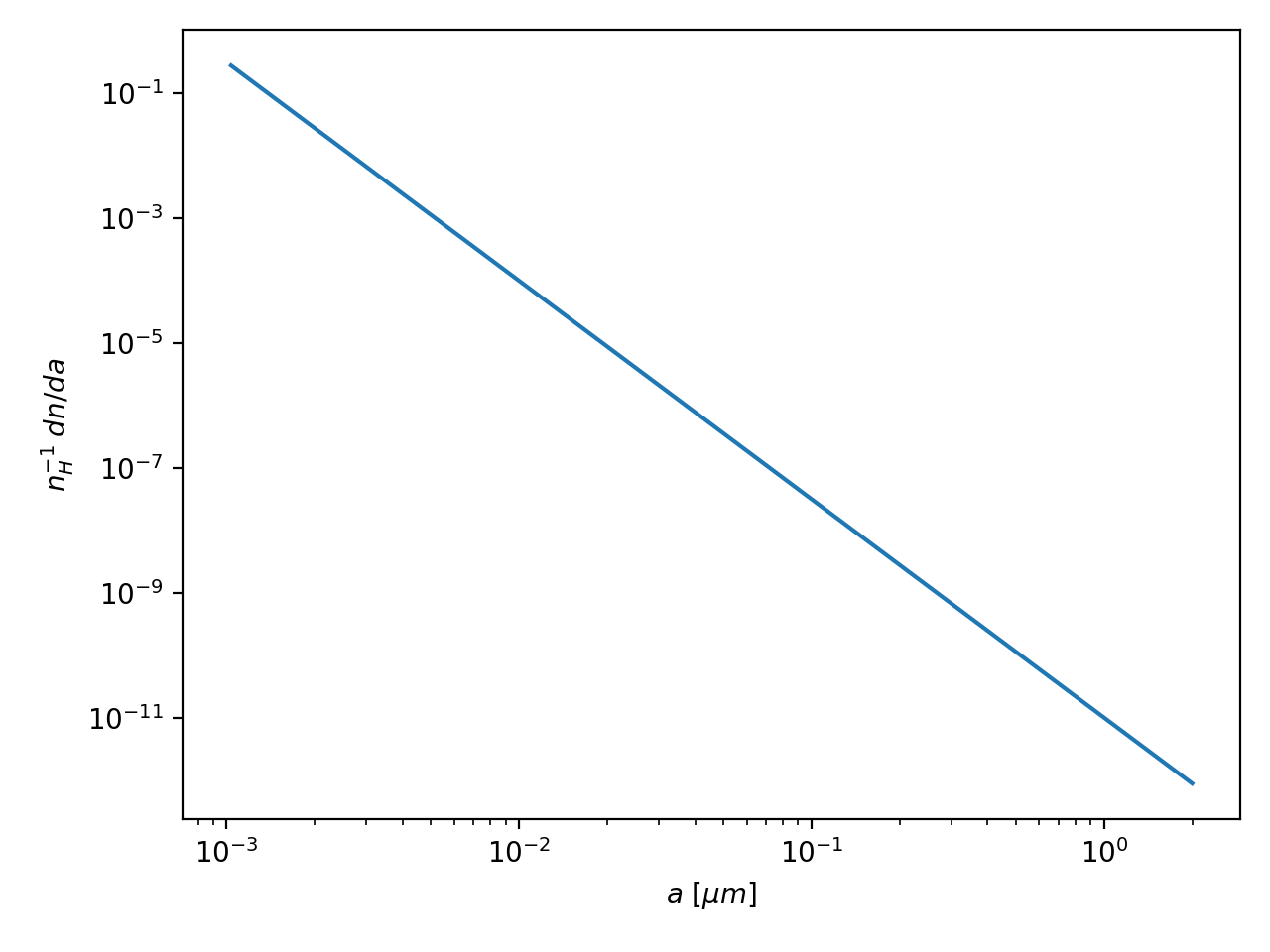
The commonly used Mathis, Rumpl, & Nordsieck (1977) size distribution is a powerlaw of the form:

\[\begin{split}\frac{dn}{da} = \left\{ \begin{array}{ll} C a ^{-\alpha} & a_{min} \leq a \leq a_{max} \\ 0 & a < a_{min} \\ 0 & a > a_{max} \\ \end{array} \right.\end{split}\]

where \(C\) is the amplitude, \(a\) is the grain radius, \(\alpha\) is the powerlaw index, and \(a_{min}\)/\(a_{max}\) give the min/max grain radii. A plot of an MRN size distribution with \(C = 1\times 10^{-25}\), \(\alpha = 3.5\), \(a_{min} = 3.5\times 10^{-4}~\mu m\), and \(a_{max} = 2~\mu m\) is shown below.

(Source code, png, hires.png, pdf)

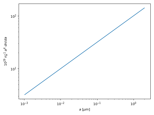
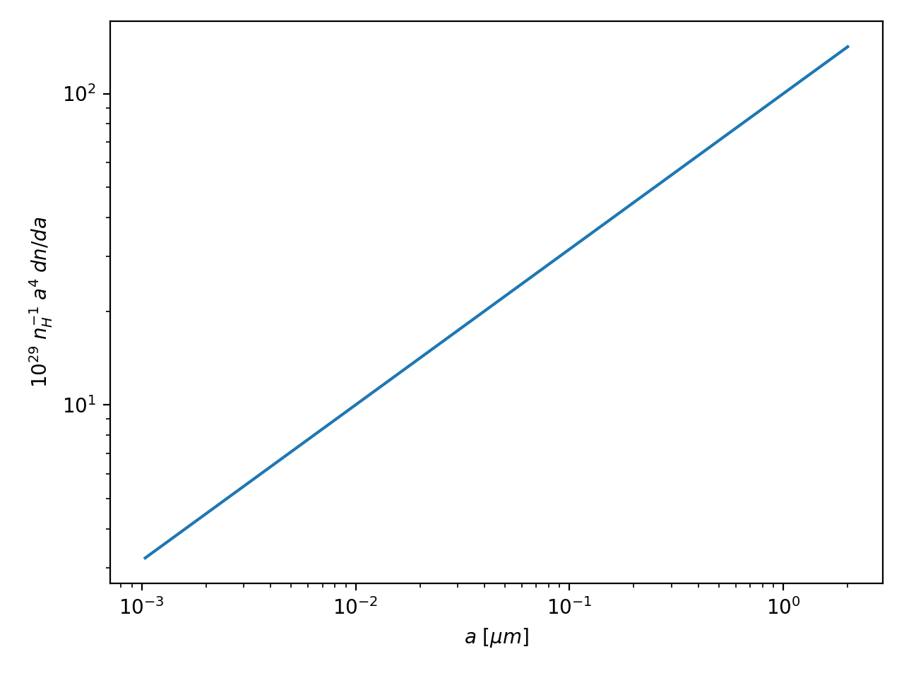
The same example size distributions are shown in a 2nd plot below where the detailed wiggles in the overall powerlaw are emphasized by multiplying by \(a^4\).

(Source code, png, hires.png, pdf)

WD

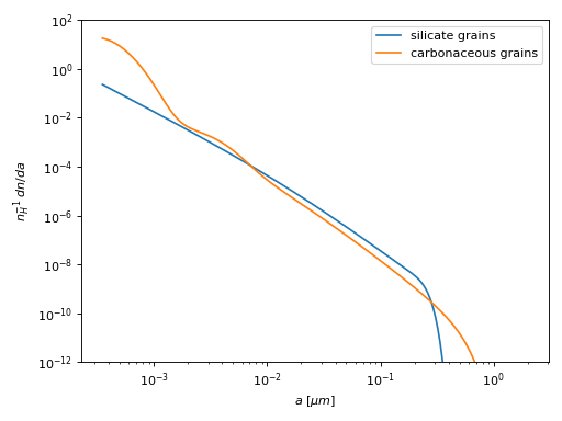
Weingartner & Draine (2001) size distributions are the referenced paper. Combining the equations from the paper results in a general form that applies to both carbonaceous and silicate grains. In the equation below, the first term provides a curved power law, the 2nd term \(D(a)\) is the sum of two log-normal functions (only used for carbonaceous grains), and all is multiplied by \(G(a)\) that results in an exponential cutoff at large grain radii.

\[\frac{dn}{da} = \left[ \frac{C}{a} \left( \frac{a}{a_t} \right)^\alpha F(a; \beta, \alpha) + D(a) \right] G(a)\]

where

\[\begin{split}F(a; \beta, \alpha) = \left\{ \begin{array}{ll} 1 + \beta a /a_t, & \beta \geq 0 \\ (1 - \beta a/a_t)^{-1} & \beta < 0 \end{array} \right.\end{split}\]

and

\[\begin{split}G(a) = \left\{ \begin{array}{ll} 1, & 0.35~\mathrm{nm} < a < a_t \\ \mathrm{exp} \left\{ -[(a - a_t)/a_c]^3 \right\} & a > a_t \end{array} \right.\end{split}\]

For silicate grains \(D(a) = 0\). For carbonaceous grains,

\[D(a) = \sum_{i=1}^2 \frac{B_i}{a} \mathrm{exp} \left\{ -\frac{1}{2} \left[ \frac{ln(a/a_{0,i})}{\sigma} \right]^2 \right\}\]

where

\[\begin{split}\begin{eqnarray} B_i & = & \frac{3}{(2\pi)^{3/2}} \frac{\mathrm{exp} (-4.5 \sigma^2)}{\rho a_{0,i}^3\sigma} \frac{b_{C,i} m_C}{1 + \mathrm{erf}(z)} \\ z & = & \frac{3 \sigma}{\sqrt{2}} + \frac{\mathrm{ln} (a_{0,i}/a_{min})}{\sigma \sqrt{2}} \\ \end{eqnarray}\end{split}\]

and for carbonaceous material \(\sigma = 0.4\), \(\rho = 2.24~\mathrm{cm}^{-3}\), \(a_{0,1} = 0.35~\mathrm{nm}\), \(a_{0,2} = 3~\mathrm{nm}\), \(a_{min} = 0.35~\mathrm{nm}\), \(b_{C,1} = 0.75 b_C\), \(b_{C,2} = 0.25 b_C\), and \(m_C\) is the mass of a carbon atom. Finally, \(b_C\) is the total C abundance in the two log-normal functions.

Example silicate and carbonaceous WD size distributions are shown below.

For the silicate grains, \(C = 1.33\times 10^{-11}\), \(a_t = 171~\mathrm{nm}\), \(\alpha = -1.41\), \(\beta = -11.5\), and \(a_c = 100~\mathrm{nm}\).

For the carbonaceous grains \(C = 4.15\times 10^{-11}\), \(a_t = 8.37~\mathrm{nm}\), \(\alpha = -1.91\), \(\beta = -0.125\), \(a_c = 499~\mathrm{nm}\), \(b_C = 3\times 10^{-5}\).

(Source code, png, hires.png, pdf)

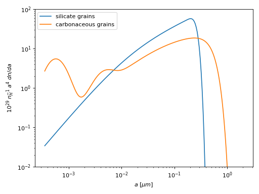
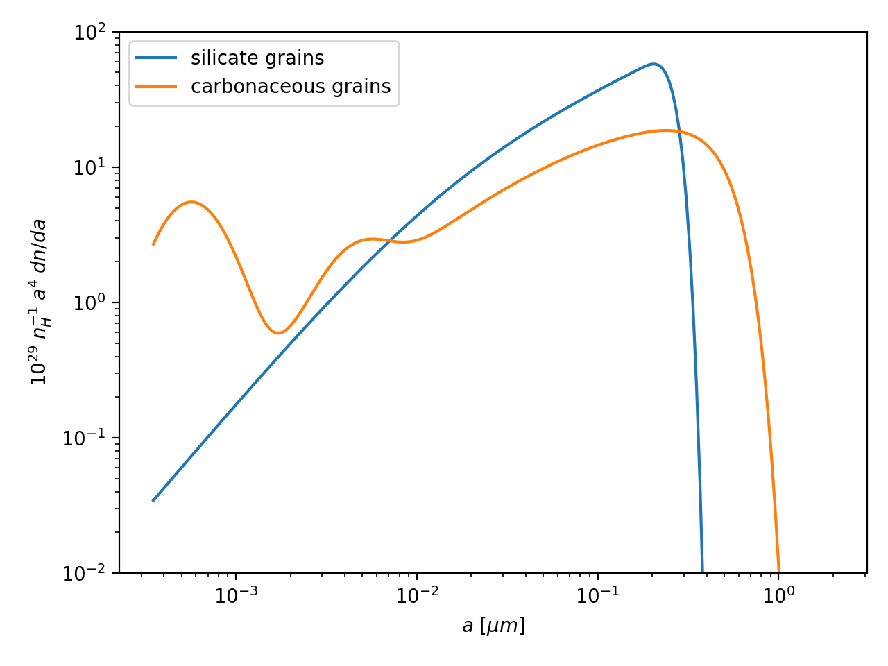
The same example size distributions are shown in a 2nd plot below where the detailed wiggles in the overall powerlaw are emphasized by multiplying by \(a^4\).

(Source code, png, hires.png, pdf)